FIELD ANALYSIS
Field Analysis
The true distribution of token efficiency across the operator field.
The true distribution of token efficiency. 1,498 AI operators, outliers separated. Volume ranked. Yield revealed.
Operator Center of Mass: 1,498 operators. Median of ratios.
Statistical Details▾
Interquartile Ranges
| Metric | Q1 | Q3 | IQR |
|---|---|---|---|
| Yield | 0.53 | 7.52 | 6.99 |
| Leverage | 9.7 | 41.2 | 31.5 |
| Velocity | 0.05 | 0.19 | 0.14 |
| SNR | 0.049 | 0.159 | 0.110 |
Benford's Law chi-square
| Pillar | χ² | Verdict |
|---|---|---|
| Input | 1.65 | PASS |
| Output | 5.54 | PASS |
| Cache Read | 4.09 | PASS |
| Cache Write | 5.47 | PASS |
| Total | 0.77 | PASS |
Critical value: χ² < 15.51 (df=8, p=0.05)
Volume ≠ Yield
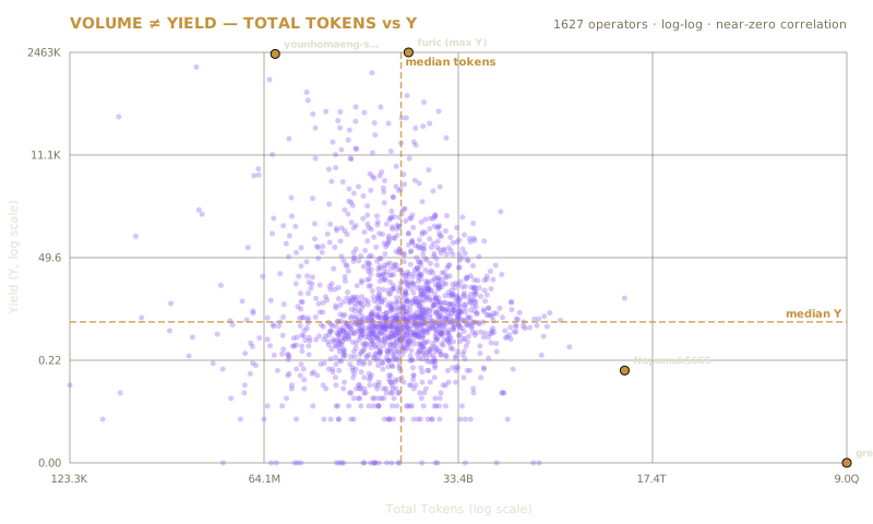
Public token-volume leaderboards rank by total token volume. SigRank ranks by yield — how efficiently an operator converts input tokens into output tokens using cache compounding. These two rankings have almost zero correlation. The operator with the most tokens (9 quadrillion) has a yield of 0. The operator with the highest yield (2.46M) ranks #697 by volume. Volume alone is noise. Yield is signal.
The scatter plot above makes this visible. The median lines divide the field into four quadrants — and the top-right (high volume, high yield) is nearly empty. The highest-yield operators cluster in the bottom-right: modest token spend, extraordinary efficiency. This is the ghost-rank phenomenon, explored below.
The Token Cascade

The median operator puts in 238M tokens of fresh input. They produce 24M tokens of output. They write 72M tokens to cache. And they read 4.77B tokens from cache. That last number is the harvest: 20.5x the seed. This is leverage. The cascade is not a chain of amplifications. It is a seed (input), a tiny sprout (output), a small store (cache write), and a massive harvest (cache read).
The operating ratio compresses this into one fingerprint: C : I : O = 19 : 1 : 0.09. For every 1 token of fresh input, the median operator reads 19 from cache and produces 0.09 output. Yield is what happens when cache compounding meets output production.
The SNR Separation
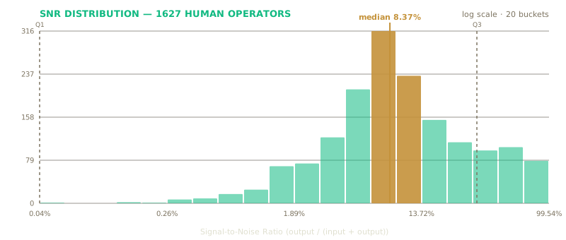
Signal-to-Noise Ratio (SNR) = output / (input + output). It measures what fraction of your interaction produced actual output versus prompt overhead. Outliers have SNR near zero. Humans have SNR above .05. One number separates signal producers from token burners.
The histogram shows the field clustering tightly around the median SNR of 0.084. The IQR fences (dashed lines) bracket the middle 50% of operators. The long tail to the right — operators with SNR above .10 — are the ghost-rank operators: they produce disproportionate output from minimal input.
Leverage × Velocity
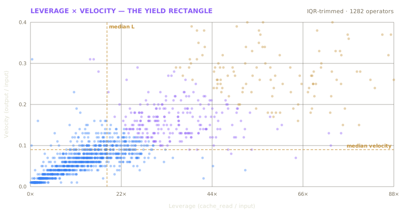
Leverage (cache_read / input) measures how much cached context amplifies each fresh input token. Velocity (output / input) measures how much the model generates per token of fresh context. Together, they define the yield rectangle — the area of leverage × velocity approximates how efficiently an operator turns cached knowledge into produced signal.
The median crosshair divides the field. Operators in the top-right quadrant — high leverage and high velocity — are the architectural elite. They read deeply from cache and produce rapidly. The bottom-left cluster (low leverage, low velocity) represents the volume-burning majority: fresh input, minimal caching, slow output.
Platform Dominance
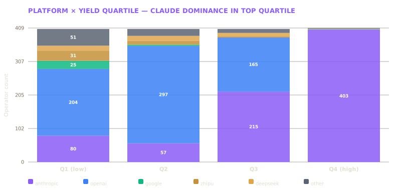
Anthropic-primary operators dominate the top yield quartile — 98.5% of the highest-yield operators use Claude as their primary platform. This isn't coincidence: Anthropic's mature prompt caching infrastructure produces higher cacheRead values, which directly drives yield.
The adoption chart shows raw volume — OpenAI and Anthropic lead in total operator count. But the quartile breakdown reveals the efficiency story: OpenAI dominates the bottom quartiles (high volume, low yield), while Anthropic owns the top. The platform you choose shapes the ceiling of your yield architecture.
Cascade Composition
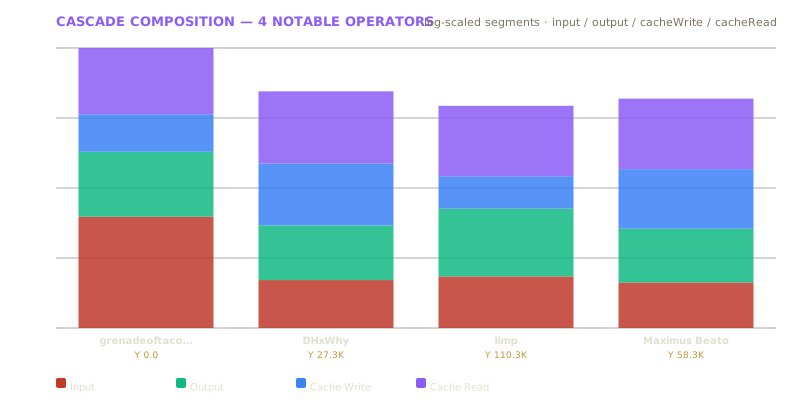
Four notable operators, four radically different cascade architectures. The stacked bars show how each operator composes their token spend across the four pillars: input (fresh tokens), output (produced signal), cache write (context stored), and cache read (context reused). The outlier at left burns input with zero cache. The high-yield operators at right are dominated by cache read — they reuse context, not burn it.
These operators illustrate the yield spectrum. See their full profiles on the Hall of Signal and learn how the metrics are computed on the methodology page.
Yield Quartile Box Plots
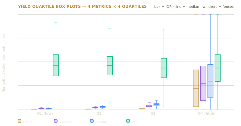
The box plots break down four metrics — yield, leverage, velocity, and SNR — across the four yield quartiles. The progression is stark: leverage jumps from a median of ~5× in Q1 to ~200× in Q4. Velocity climbs from 0.03 to nearly 1.0. But SNR stays flat across all quartiles — the signal density of output doesn't change. What changes is how much cached context amplifies that output.
This is the architectural insight: high-yield operators don't produce denser signal — they produce more signal from the same density by leveraging cache. The yield gap is a leverage gap, not a talent gap.
Where 80% of Operators Live

80% of operators have a yield between 0.37 and 233.12. The median is 1.68. The distribution is heavily right-skewed (power-law), which is why the median is used instead of the mean.
The yield distribution is heavily right-skewed. 80% of operators fall within the shaded band. The long tail to the right is where the AMPLIFIERS and CONVERGENT operators live. The bulk of the field clusters near the median. This is why the median is used instead of the mean: the mean is pulled by outliers, the median reflects where operators actually are.
The average-user anchor. The median yield of 1.68 sits close to the Artificial Analysis modeled “average AI user” baseline of 1.75 (the 7:2:1 cache-read : cache-write : input ratio). But the composition is very different: the real field has 18.6× leverage vs the model's 3.5× — real operators read far more cache — but only 0.09 velocity vs the model's 0.50 — they produce less output per input token. Cache-heavy, output-light. Net yield is close to the modeled average; the path there is not. See the Four Degrees of Leverage for the full cascade.
Where Are You?

Median yield is 1.68. You are probably here. Claim your profile to see exactly where you land
The percentile ladder shows the yield thresholds for each tier. The median is where most operators land. The top 1% is where cache architecture becomes an art form. If you use AI coding agents, you are probably near the median. Claim your profile to see exactly where you fit.
Ghost Ranks: The Hidden Operators
Ghost-rank operators are invisible on volume-based leaderboards but dominate yield-based rankings. They use fewer tokens but achieve higher output efficiency. These are the operators worth recruiting — they have skill, not just spend.
The data reveals 50 ghost-rank operators — above median yield but with volume ranks in the hundreds or thousands. Their median volume rank is 1355, meaning they are buried deep on any volume leaderboard. But their yield values reach into the hundreds of thousands. Volume metrics hide them. Yield metrics find them.
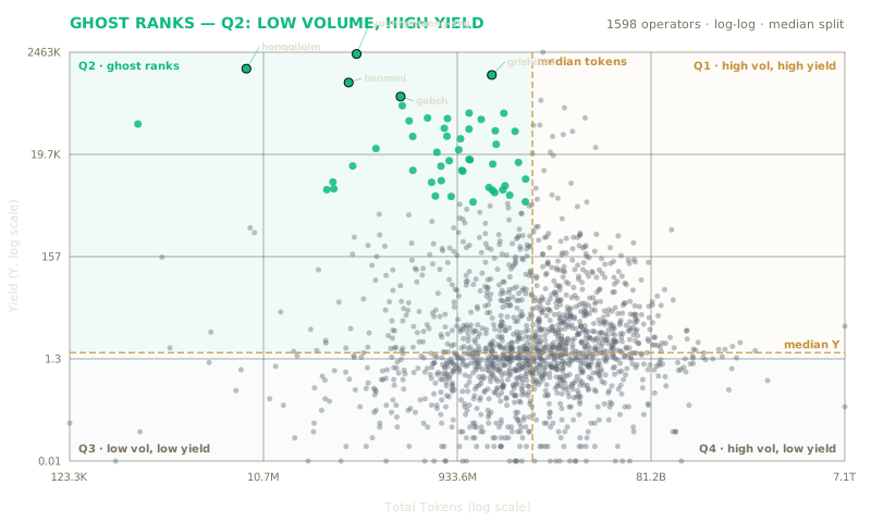
The quadrant chart above plots every operator on a log-log grid of total tokens versus yield. The dashed gold lines mark the median on each axis, splitting the field into four quadrants. Q2 — the top-left, low volume and high yield — is the ghost-rank region, highlighted in cyan. These operators would be invisible on any volume-ranked leaderboard, yet they dominate on yield. They are the operators worth recruiting.
| Handle | Tokscale Rank | Yield (Υ) | Total Tokens | Platform |
|---|---|---|---|---|
| operator-24f2c607 | #1,574 | 2266.0K | 91.7M | anthropic |
| operator-9b52fcca | #1,618 | 1130.0K | 7.2M | anthropic |
| operator-361a8867 | #1,142 | 839.6K | 2.1B | anthropic |
| operator-c081fff6 | #1,584 | 587.0K | 76.3M | anthropic |
| operator-990f3b85 | #1,509 | 302.1K | 253.0M | anthropic |
| operator-3413b7e4 | #1,505 | 196.9K | 263.2M | anthropic |
| operator-02598a10 | #1,278 | 138.6K | 1.2B | anthropic |
| operator-1f71d770 | #1,041 | 137.7K | 2.7B | anthropic |
| operator-8a2bf848 | #1,459 | 109.8K | 471.1M | anthropic |
| operator-f609f5a2 | #1,389 | 107.4K | 745.5M | anthropic |
| operator-b22c9f7d | #1,207 | 103.0K | 1.6B | anthropic |
| operator-8e538cca | #1,490 | 95.6K | 308.2M | anthropic |
| operator-9f3ee1ed | #1,626 | 82.6K | 0.6M | anthropic |
| operator-e8d1aa7a | #1,408 | 67.4K | 692.4M | anthropic |
| operator-9516800c | #1,279 | 65.1K | 1.2B | anthropic |
| operator-2cba35a1 | #1,113 | 59.8K | 2.2B | anthropic |
| operator-e4a93bb4 | #956 | 58.6K | 3.5B | anthropic |
| operator-e8695d75 | #1,391 | 46.4K | 736.1M | anthropic |
| operator-49d5af41 | #1,486 | 45.9K | 335.0M | anthropic |
| operator-648eb52c | #1,326 | 41.3K | 1.0B | anthropic |
Showing 20 of 50 ghost-rank operators.
Claim your profile →Build Archetypes
The field separates into 10 build archetypes across four families: Convergence, Generation, Reuse Depth, and Active Construction. CONVERGENT is checked first and pulls out operators who are elite on all three derived dimensions (leverage, velocity, construction). KINETIC captures high-velocity generation. The Construction branch captures active context builders. The Reuse Depth branch captures passive context reusers. Each type is defined by a different primary dimension of the token cascade.
CONVERGENT
n=104 (6.6%)
Deep reuse, active construction, and high generation rise together. A rare composition where all three operating axes are elevated without the usual tradeoffs.
Convergence · P80 on all 3 axes (leverage + velocity + construction)
KINETIC
n=113 (7.1%)
Generation has broken out. Output approaches or exceeds fresh input, making transmission the defining feature of the composition.
Generation · velocity >= 0.80
INPUT-BOUND
n=108 (6.8%)
Fresh input still carries most of the workload. Little prior context is returning, so each cycle depends heavily on new input.
Reuse Depth · leverage < 5
PRIMING
n=149 (9.4%)
Reuse is beginning to form. Prior context is returning, but the system has not yet developed deep leverage.
Reuse Depth · leverage 5–10
CONTEXTUAL
n=186 (11.7%)
Retained context is now materially supporting the workflow. Reuse is established, while active construction remains limited.
Reuse Depth · leverage 10–15, passive
DEEP READER
n=169 (10.7%)
Strong accumulated context is carrying the workflow. The operator draws deeply from retained context while creating relatively little new context.
Reuse Depth · leverage 15–23, passive
ARCHIVIST
n=186 (11.7%)
Extreme reuse of accumulated context. A deep context library carries the system while new construction remains limited.
Reuse Depth · leverage >= 23, passive
BUILDER
n=278 (17.5%)
Active context construction has begun. The system is creating material for future reuse while leverage is still developing.
Active Construction · construction >= 0.02, leverage < 30
RECURSIVE
n=132 (8.3%)
New context is being built on top of an already substantial reusable base. Construction and reuse are now feeding the same operating loop.
Active Construction · construction >= 0.02, leverage 30–50
AMPLIFIER
n=161 (10.2%)
Deep reuse and active construction are operating together at scale. Existing context produces new work that expands the context available for future cycles.
Active Construction · construction >= 0.02, leverage >= 50
Build archetypes are deterministic classifications based on token cascade dimensions — leverage (cache_read/input), velocity (output/input), and construction (cache_write/cache_read). Each type is defined by a different primary dimension. CONVERGENT is checked first and pulls out operators who are elite on all three axes.
Outlier Detection
Outlier Exclusion Zones
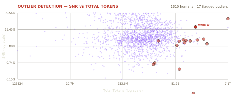
Outliers are not deleted. They get their own category and rank against each other. They just do not set the numbers for the Operator Center of Mass.
A 6-signal outlier-likelihood score checks throughput, cache usage, model concentration, and session evidence. 130 statistical outliers were separated from this historical field distribution. The input/total analysis also distinguishes productive high-reuse signatures from replay and input-dump anomalies. Those screens measure token-flow structure; workflow-mode labels need their own evidence.
The scatter plot shows one outlier pattern in the bottom-right: massive token volume with near-zero SNR, where input dominates and little output appears. Other high-reuse outliers have substantial output and cache construction; they are a different operating signature. The 6-signal score flags records for closer analysis rather than proving an operator's identity or level of human involvement.
This is why the Four Degrees chart's columns are honest: the 130 outliers are separated before the median is computed. Without separation, the top outlier alone skews the field average by 248,000%. The median is immune. Read the full analysis or see the Four Degrees of Leverage to see how the clean median compares to the modeled average.